|
| Digital camera.11.9 |
Data sets are usually available in the form of a file or a set of files. In order to manipulate the data with a general-purpose language, we must read the data from a file and store it in a data structure that our language understands (e.g., a data frame). R provides many functions for reading data in a wide variety of file formats.
Any function that works with a file requires a precise description of the name of the file and the location of the file.
A file name is just a string, e.g., "pointnemotemp.txt". Specifying the location of a file can involve a path, which describes a location on a hard drive, or a URL describing an internet location.
The best way to specify a path in R is via the file.path() function because this avoids the differences between path descriptions on different operating systems.
The file.choose() function can be used to allow interactive selection of a file. This is particularly effective on Windows because it provides a familiar file selection dialog box.
Some data management tasks do not involve the contents of files at all, but are only concerned with reorganising entire sets of files. Examples include moving files between directories and renaming files.
These are tasks that are commonly performed via a GUI that is provided by the operating system, for example, Windows Explorer on Windows or the Finder on a Macintosh. However, as with most tasks we have discussed, if a large number of files are involved it is much more efficient and much less error-prone to perform these tasks by writing a script.
R provides functions for basic file manipulation, including list.files() for listing the files in a directory, file.copy() for moving files between directories, and file.rename() for renaming files.
Digital camera.11.9
Digital cameras have revolutionised photography. No longer are we restricted to a mere 26 shots per film; it is now common to be able to take one hundred photographs or more on a basic camera. No longer do we have to process a film in order to find out whether we have captured the perfect shot; we can preview photographs instantly and photos can be viewed in all their glory with a simple download to a computer. Printing photographs is instantaneous and sharing photographs with friends and family is almost too easy.
Unfortunately, digital cameras have also ruined many people's lives. Suddenly, every amateur snapper has to deal with thousands of computer files and not everyone is equipped for this task.
The international standard for expressing dates (ISO 8601) specifies a YYYY-MM-DD format (four-digit year, two-digit month, and two-digit day). For example, the set of photos taken on christmas day with the mother in law could be named 2006-12-25.
If we name our digital photograph directories by international standard date then we can easily list them in date order (natural alphabetical order achieves this) and then at least immediately focus in on the appropriate period of time to locate a particular photograph of interest.
We can always still add extra mnemonics to the end of the filename, for example, 2007-12-25-ChristmasWithMotherInLaw in order to make finding the right photos even quicker.
In practice, even with this sort of knowledge, what tends to happen is that photos end up in files that are named in all sorts of different ways. In this section, we will look at how to clean up such a mess.
The list.files() function can be used to create a list of file names for a given directory. Here is a list of directories that contain some of my digital photos.
> directories <- list.files("Photos")
> directories
 [1] "061111"  "061118"  "061119"  "061207"  "061209"
 [6] "061216"  "061219"  "061231"  "06Nov05" "06Oct05"
[11] "06Oct15" "06Oct28" "06Sep17" "070103"  "070105"
[16] "070107"  "070108"  "070113"  "070114"  "070117"
[21] "070202"  "070218"  "070223"  "070303"  "070331"
Unfortunately, the naming of these directories has been a little undisciplined. Many of the directories are named using something like the method outlined in Section 11.6.3: a YYMMDD format where year, month, and day are all represented by two-digit integers. However, some of the earlier directories used a slightly different format: YYmmmDD, where year and day are two-digit integers, but month is a three-character abbreviated name.
We can make the naming consistent via a simple search-and-replace operation on the directory names. This example uses the sub() function to replace "Nov" with "11", "Oct" with 10, and so on, in all directory names.11.10
> newDirs <- sub("Nov", "11", directories)
> newDirs <- sub("Oct", "10", newDirs)
> newDirs <- sub("Sep", "09", newDirs)
> newDirs
 [1] "061111" "061118" "061119" "061207" "061209" "061216"
 [7] "061219" "061231" "061105" "061005" "061015" "061028"
[13] "060917" "070103" "070105" "070107" "070108" "070113"
[19] "070114" "070117" "070202" "070218" "070223" "070303"
[25] "070331"
Now that the directory names are all in the same format, we can easily convert them to dates.
> dateDirs <- as.Date(newDirs, format="%y%m%d")
> dateDirs
 [1] "2006-11-11" "2006-11-18" "2006-11-19" "2006-12-07"
 [5] "2006-12-09" "2006-12-16" "2006-12-19" "2006-12-31"
 [9] "2006-11-05" "2006-10-05" "2006-10-15" "2006-10-28"
[13] "2006-09-17" "2007-01-03" "2007-01-05" "2007-01-07"
[17] "2007-01-08" "2007-01-13" "2007-01-14" "2007-01-17"
[21] "2007-02-02" "2007-02-18" "2007-02-23" "2007-03-03"
[25] "2007-03-31"
Now we can loop over the directory names and change the original name to one based on the date in a standard format. This is the crucial step in this task; a script to perform file renaming automatically, rather than with a mouse via a GUI.
> numDirs <- length(directories)
> for (i in 1:n) {
       file.rename(file.path("Photos", directories[i]),
                   file.path("Photos", dateDirs[i]))
   }
The files are all now in a common, standard format.
> list.files("Photos")
 [1] "2006-09-17" "2006-10-05" "2006-10-15" "2006-10-28"
 [5] "2006-11-05" "2006-11-11" "2006-11-18" "2006-11-19"
 [9] "2006-12-07" "2006-12-09" "2006-12-16" "2006-12-19"
[13] "2006-12-31" "2007-01-03" "2007-01-05" "2007-01-07"
[17] "2007-01-08" "2007-01-13" "2007-01-14" "2007-01-17"
[21] "2007-02-02" "2007-02-18" "2007-02-23" "2007-03-03"
[25] "2007-03-31"
One final step is recommended in this example. The act of renaming a file is a one-way trip. The original file names are lost. If we ever need to be able to go back to the original file names, for example, if we want to match the new directories with old versions of the directories from a backup, we should record both the old and the new file names. This is easily accomplished in the following code, which writes the old an new filenames into a text file.
> write.table(data.frame(old=directories,
                          new=dateDirs),
               file="rename.txt",
               quote=FALSE, row.names=FALSE)
R has functions for reading in each of the standard plain text formats, each of which creates a data frame from the contents of the text file:
There is also a function readLines() that creates a character vector from a text file, where each line of the text file is a separate element of the vector. This is useful for processing the text within a file (see Section 11.8).
Recall the plain text file of temperature data obtained from NASA's Live Access Server for the Pacific Pole of Inaccessibility (see Section 1.1; Figure 11.6 reproduces Figure 1.2 for convenience). How can we load this temperature information into R?
|
            VARIABLE : Mean TS from clear sky composite (kelvin)
            FILENAME : ISCCPMonthly_avg.nc
            FILEPATH : /usr/local/fer_dsets/data/
            SUBSET   : 93 points (TIME)
            LONGITUDE: 123.8W(-123.8)
            LATITUDE : 48.8S
                      123.8W
                       23
16-JAN-1994 00 /  1:  278.9
16-FEB-1994 00 /  2:  280.0
16-MAR-1994 00 /  3:  278.9
16-APR-1994 00 /  4:  278.9
16-MAY-1994 00 /  5:  277.8
16-JUN-1994 00 /  6:  276.1
...
|
One way to view the format of the file in Figure 1.2 is that the data start on line 9 and data values are separated by whitespace. We will use the read.table() function to read the Point Nemo temperature information and create a data frame.
> pointnemotemp <-
       read.table("pointnemotemp.txt", skip=8,
                  colClasses=c("character",
                    "NULL", "NULL", "NULL",
                    "numeric"),
                  col.names=c("date", "", "", "", "temp"))
> pointnemotemp
         date  temp
1 16-JAN-1994 278.9
2 16-FEB-1994 280.0
3 16-MAR-1994 278.9
4 16-APR-1994 278.9
5 16-MAY-1994 277.8
6 16-JUN-1994 276.1
...
By default, read.table() assumes that the text file contains a data set with one case on each row and that each row contains multiple values, with each value separated by white space. The skip argument is used to ignore the first few lines of a file when, for example, there is header information or metadata at the start of the file before the actual data values.
A data frame is produced with a variable for each column of values in the text file. The types of variables are determined automatically; if a column only contains numbers, the variable is numeric, otherwise, the variable is a factor. The colClasses argument allows us to control the types of the variables explicitly. In this case, we have forced the first variable to be just text (these values are dates, not categories). There are five columns of values in the text file (treating white space as a column break), but we are not interested in the middle three, so we use "NULL" to indicate that these columns should not be included in the data frame.
In many cases, the names of the variables will be included as the first line of a text file (the header argument can be used to read variable names from such a file). In this case, we must provide the variable names explicitly, using the col.names argument.
The read.table() function is quite flexible and can be used for a variety of plain text formats. If the format is too complex for read.table() to handle, the scan() function may be able to help; this function is also useful for reading in very large text files because it is faster than read.table(). Some other functions are designed specifically for more standard plain text formats. The function read.fwf() is for files with a fixed-width format. If the format of the file is comma-separated values (CSV), then read.csv() can be used.
In cases where the file format is complex, another option is to preprocess the file to produce a more convenient format. This is most easily done by reading the original file as just a vector of text using the function readLines(), rearranging the text, and writing the new text to a new file using writeLines(). The following code uses this approach to reformat the Point Nemo temperature data.
> temperatureText <- readLines("pointnemotemp.txt")
> temperatureText
 [1] "             VARIABLE : Mean TS from clear sky composite (kelvin)"
 [2] "             FILENAME : ISCCPMonthly_avg.nc"
 [3] "             FILEPATH : /usr/local/fer_dsets/data/"
 [4] "             SUBSET   : 93 points (TIME)"
 [5] "             LONGITUDE: 123.8W(-123.8)"
 [6] "             LATITUDE : 48.8S"
 [7] "                       123.8W "
 [8] "                        23"
 [9] " 16-JAN-1994 00 /  1:  278.9"
[10] " 16-FEB-1994 00 /  2:  280.0"
...
Having read the data in with readLines(), the variable temperatureText contains a vector with a string for each line of the file.
> keepRows <- temperatureText[-(1:8)]
> keepRows
[1] " 16-JAN-1994 00 /  1:  278.9"
[2] " 16-FEB-1994 00 /  2:  280.0"
[3] " 16-MAR-1994 00 /  3:  278.9"
[4] " 16-APR-1994 00 /  4:  278.9"
[5] " 16-MAY-1994 00 /  5:  277.8"
[6] " 16-JUN-1994 00 /  6:  276.1"
...
We drop the first 8 elements of the vector, which are the first 8 lines of the file (Section 11.7 provides more details on subsetting and rearranging data structures).
> keepCols <- sub(" 00 / ..: ", "", keepRows)
> keepCols
[1] " 16-JAN-1994 278.9" " 16-FEB-1994 280.0"
[3] " 16-MAR-1994 278.9" " 16-APR-1994 278.9"
[5] " 16-MAY-1994 277.8" " 16-JUN-1994 276.1"
...
The string manipulation step uses the sub() function to delete the parts of each row that we are not interested in (Section 11.8 provides more details on string processing tasks). Finally, we write the new text to a new file using writeLines() (see Figure 11.7).
> writeLines(keepCols, "pointnemoplain.txt")
|
16-JAN-1994 278.9 16-FEB-1994 280.0 16-MAR-1994 278.9 16-APR-1994 278.9 16-MAY-1994 277.8 16-JUN-1994 276.1 16-JUL-1994 276.1 16-AUG-1994 275.6 ... |
With this new file, reading the data into a data frame is more straightforward: we no longer have header lines to skip and we no longer have extra columns to ignore. Instead of using the colClasses argument, we use the as.is argument to specify that the non-numeric column should be left as text, not converted to a factor.
> pointnemotemp <-
       read.table("pointnemoplain.txt", as.is=TRUE,
                  col.names=c("date", "temp"))
The network packet data set described in Section 7.4.4
contains measurements of the time that a packet of information
arrives at a location in a network. These measurements are the number
of seconds since January ![]() 1970 and are recorded to the nearest
10,000
1970 and are recorded to the nearest
10,000![]() of a second, so they are very large
and very precise numbers. Figure 11.8
shows the data stored in a plain text format (the time measurements
are in the first column).
of a second, so they are very large
and very precise numbers. Figure 11.8
shows the data stored in a plain text format (the time measurements
are in the first column).
|
1156748010.47817 60 1156748010.47865 1254 1156748010.47878 1514 1156748010.4789 1494 1156748010.47892 114 1156748010.47891 1514 1156748010.47903 1394 1156748010.47903 1514 1156748010.47905 60 1156748010.47929 60 ... |
The XML package contains functions for reading XML files into R. The object that is created is complex and must be worked with using special functions from the XML package.
The Point Nemo temperature data can also be represented in an XML format (see Figure 11.9).
|
<?xml version="1.0"?>
<temperatures>
    <variable>Mean TS from clear sky composite (kelvin)</variable>
    <filename>ISCCPMonthly_avg.nc</filename>
    <filepath>/usr/local/fer_dsets/data/</filepath>
    <subset>93 points (TIME)</subset>
    <longitude>123.8W(-123.8)</longitude>
    <latitude>48.8S</latitude>
    <case date="16-JAN-1994" temperature="278.9" />
    <case date="16-FEB-1994" temperature="280" />
    <case date="16-MAR-1994" temperature="278.9" />
    <case date="16-APR-1994" temperature="278.9" />
    <case date="16-MAY-1994" temperature="277.8" />
    <case date="16-JUN-1994" temperature="276.1" />

    ...

</temperatures>
|
This file can be read into R quite easily.
> library(XML)
> nemoDoc <- xmlTreeParse("pointnemotemp.xml")
However, the nemoDoc object is relatively complex so we must
use special functions to extract information from it. For example,
the xmlRoot() function extracts the “root” element from the
document. For each element, it is simple to extract
the name of the element using xmlName().
In this case, the root element of the document is a
temperatures element.
> nemoDocRoot <- xmlRoot(nemoDoc)
> xmlName(nemoDocRoot)
[1] "temperatures"
The root element is itself quite complex; in particular, it is hierarchical to reflect the nested nature of the XML elements in the original document. The xmlChildren() element extracts the elements that are nested within an element.
> nemoDocChildren <- xmlChildren(nemoDocRoot)
> head(nemoDocChildren)
$variable
<variable>Mean TS from clear sky composite (kelvin)</variable>

$filename
<filename>ISCCPMonthly_avg.nc</filename>

$filepath
<filepath>/usr/local/fer_dsets/data/</filepath>

$subset
<subset>93 points (TIME)</subset>

$longitude
<longitude>123.8W(-123.8)</longitude>

$latitude
<latitude>48.8S</latitude>
For an individual element, the function xmlAttrs() extracts the attributes of the element and xmlValue() extracts the contents of the element.
The first child element describes the variable in the data set.
> nemoDocChildren[[1]]
<variable>Mean TS from clear sky composite (kelvin)</variable>
> xmlValue(nemoDocChildren[[1]])
[1] "Mean TS from clear sky composite (kelvin)"
The seventh child element is the first actual data value.
> nemoDocChildren[[7]]
<case date="16-JAN-1994" temperature="278.9"/>
> xmlAttrs(nemoDocChildren[[7]])
         date   temperature
"16-JAN-1994"       "278.9"
Some of the concepts from Section 11.7 for working with list objects and from Section and 11.10 for writing R functions will be needed to become fully proficient with the XML package. For example, extracting all of the temperature data values requires writing a new function which then needs to be called on each element of the document root.
> temperatureFun <- function(x) {
       if (xmlName(x) == "case") {
           xmlAttrs(x)["temperature"]
       }
   }
> nemoDocTemps <-
       as.numeric(unlist(xmlApply(nemoDocRoot,
                                  temperatureFun)))
> nemoDocTemps
 [1] 278.9 280.0 278.9 278.9 277.8 276.1 276.1 275.6 275.6
[10] 277.3 276.7 278.9 281.6 281.1 280.0 278.9 277.8 276.7
[19] 277.3 276.1 276.1 276.7 278.4 277.8 281.1 283.2 281.1
[28] 279.5 278.4 276.7 276.1 275.6 275.6 276.1 277.3 278.9
[37] 280.5 281.6 280.0 278.9 278.4 276.7 275.6 275.6 277.3
[46] 276.7 278.4 279.5 282.2 281.6 281.6 280.0 278.9 277.3
[55] 276.7 276.1 276.1 276.1 277.8 277.3 278.4 284.2 279.5
[64] 277.3 278.4 275.0 275.6 274.4 275.6 276.7 276.1 278.4
[73] 279.5 279.5 278.9 277.8 277.8 275.6 275.6 275.0 274.4
[82] 275.6 277.3 278.4 281.1 283.2 281.1 279.5 277.3 276.7
[91] 275.6 274.4 275.0
As discussed in Section 7.7, it is only possible to extract data from a binary file with an appropriate piece of software.
This obstacle is less of a problem for binary formats which are publicly documented so that it is possible to write software that can read the format. In some cases, such software has already been written and made available to the public. An example of the latter is the NetCDF software library.11.11
A number of R packages exist for reading particular formats. For example, the foreign package contains functions for reading files produced by other popular statistics software systems, such as SAS, SPSS, Systat, Minitab, and Stata. The ncdf package provides functions for reading NetCDF files.
Yet another format for the Point Nemo temperature data is as a NetCDF file. Figure 11.10) shows both a structured and an unstructured view of the raw binary file.
|
   0  :  43 44 46 01 00 00  |  CDF...
   6  :  00 00 00 00 00 0a  |  ......
  12  :  00 00 00 01 00 00  |  ......
  18  :  00 04 54 69 6d 65  |  ..Time
  24  :  00 00 00 5d 00 00  |  ...]..
  30  :  00 00 00 00 00 00  |  ......
  36  :  00 00 00 0b 00 00  |  ......
  42  :  00 02 00 00 00 04  |  ......
  48  :  54 69 6d 65 00 00  |  Time..
  54  :  00 01 00 00 00 00  |  ......
  ...
=========magicNumber 0 : 43 44 46 01 | CDF. =========numRecords 4 : 00 00 00 00 | 0 =========dimensionArrayFlag 8 : 00 00 00 0a | 10 =========dimensionArraySize 12 : 00 00 00 01 | 1 =========dim1NameSize 16 : 00 00 00 04 | 4 =========dim1Name 20 : 54 69 6d 65 | Time =========dim1Size 24 : 00 00 00 5d | 93 ... |
A NetCDF file has a flexible structure, but it is self-describing. This means that we must read the file in stages. First of all, we open the file and inspect the contents.
> library(ncdf)
> nemonc <- open.ncdf("pointnemotemp.nc")
> nemonc
file pointnemotemp.nc has 1 dimensions:
Time   Size: 93
------------------------
file pointnemotemp.nc has 1 variables:
float Temperature[Time]  Longname:Temperature
Having seen that the file contains a single variable called Temperature, we extract that variable from the file with a separate function call.
> nemoTemps <- get.var.ncdf(nemonc, "Temperature")
> nemoTemps
 [1] 278.9 280.0 278.9 278.9 277.8 276.1 276.1 275.6 275.6
[10] 277.3 276.7 278.9 281.6 281.1 280.0 278.9 277.8 276.7
[19] 277.3 276.1 276.1 276.7 278.4 277.8 281.1 283.2 281.1
[28] 279.5 278.4 276.7 276.1 275.6 275.6 276.1 277.3 278.9
[37] 280.5 281.6 280.0 278.9 278.4 276.7 275.6 275.6 277.3
[46] 276.7 278.4 279.5 282.2 281.6 281.6 280.0 278.9 277.3
[55] 276.7 276.1 276.1 276.1 277.8 277.3 278.4 284.2 279.5
[64] 277.3 278.4 275.0 275.6 274.4 275.6 276.7 276.1 278.4
[73] 279.5 279.5 278.9 277.8 277.8 275.6 275.6 275.0 274.4
[82] 275.6 277.3 278.4 281.1 283.2 281.1 279.5 277.3 276.7
[91] 275.6 274.4 275.0
When data is stored in a spreadsheet, one common approach is to save the data in a text format in order to read it into another program. This makes the data easy to read, but has the disadvantage that it creates another copy of the data, which is less efficient in terms of storage space and creates issues if the original spreadsheet is updated. At best, there is extra work to be done to update the text file as well. At worst, the text file is forgotten and the update does not get propagated to other places.
There are several packages that provide ways to directly read data from a spreadsheet into R. One example is the (Windows only) xlsReadWrite package, which includes the read.xls() function.
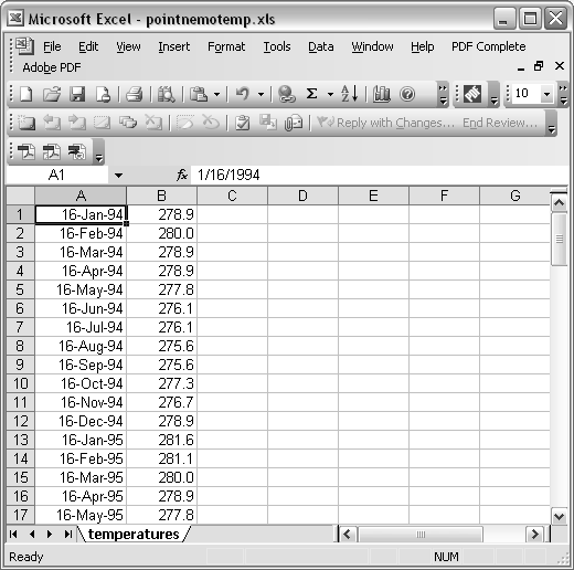
Figure 11.11 shows a screen shot of the Point Nemo temperature data stored in a Microsoft Excel spreadsheet.
These data can be read into R as follows. Notice that
the date information has come across as numbers (specifically,
the number of days since the ![]() of January 1900).
This is a demonstration of the difference between the
formatted information that we see in the display layer
of a spreadsheet and the internal format of the storage layer.
of January 1900).
This is a demonstration of the difference between the
formatted information that we see in the display layer
of a spreadsheet and the internal format of the storage layer.
> read.xls("temperatures.xls", colNames=FALSE)
      V1    V2
1  34350 278.9
2  34381 280.0
3  34409 278.9
4  34440 278.9
5  34470 277.8
6  34501 276.1
...
Very large data sets are often stored in relational database management systems. Again, a simple approach to extracting information from the database is to simply export it as text files and work with the text files. This is an even worse option for databases than it was for spreadsheets because it is more common to extract just part of a database, rather than an entire spreadsheet. This can lead to several different text files from a single database and these are even harder to maintain if the database changes.
There are packages for connecting directly to several major database management systems. Most of these packages are built on the DBI package, which defines some standard functions. Each package for a specific database system provides special behaviour for these standard functions that is appropriate for the relevant database.
The Data Expo data set (see Section 7.5.6) contains several different atmospheric measurements, all measured 72 different time periods and 576 different locations. These data have been stored in an SQLite database, with a table for location information, a table for time period information, and a table of the atmospheric measurements (see Section 9.2.2).
The following code extracts surface temperature measurements for locations on land during the first year of recordings.
> library(RSQLite)
> con <- dbConnect(dbDriver("SQLite"),
                    dbname="NASA/dataexpo")
> landtemp <-
       dbGetQuery(con,
                  "SELECT surftemp
                       FROM measure_table
                       WHERE pressure < 1000 AND
                             date < '1996-01-16'")
> dbDisconnect(con)
> head(landtemp)
  surftemp
1    272.7
2    270.9
3    270.9
4    269.7
5    273.2
6    275.6
Paul Murrell

This document is licensed under a Creative Commons Attribution-Noncommercial-Share Alike 3.0 License.