 |
General-purpose languages allow us to work with numbers, text (strings), and logical values. This section briefly describes important features of how values are represented using these basic data types, then goes on to the larger topic of how multiple values, possibly of differing types, can be stored together in data structures.
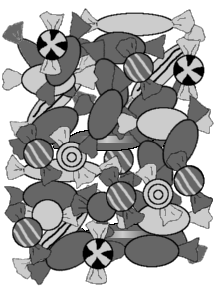
The image in Figure 11.5 shows a simple counting puzzle. The task is to count how many of each different type of candy there are in the image.
|
Our task is to record the different shapes (round, oval, or long), the different shades (light or dark), and whether there is a pattern on the candies that we can see in the image. How can this information be entered into R?
One way to enter data in R is to use the scan() function. This allows us to type data into R separated by spaces. Once we have entered all of the data, we enter an empty line to indicate to R that we have finished. We will use this to enter the different shapes:
> shapeNames <- scan(what="character")
1: round oval long
4:
Read 3 items
> shapeNames
[1] "round" "oval" "long"
Another way to enter data is using the c() function. We will use this to enter the possible patterns and shades:
> patternNames <- c("pattern", "plain")
> patternNames
[1] "pattern" "plain"
> shadeNames <- c("light", "dark")
> shadeNames
[1] "light" "dark"
All we have done so far is enter the possible values of these symbols. As we learn more about the basic R data structures below, we will add counts of how many times each shape-shade-pattern combination occurs.
One of the reasons that R is a good environment for working with data is because it works with vectors of values. Any symbol, like shapes, pattern, and shades above, can contain many values at once.
There are also many basic functions for manipulating vectors.
We have already seen the c() function for combining values together (above). Another example is the rep() function, which can be used to repeat values in a vector. We can use this function to create a symbol representing the shade for each of the candies in the image above (by my count, there are 11 light-coloured candies and 25 dark-coloured candies).
> shades <- rep(shadeNames, c(11, 25))
> shades
 [1] "light" "light" "light" "light" "light" "light" "light"
 [8] "light" "light" "light" "light" "dark"  "dark"  "dark"
[15] "dark"  "dark"  "dark"  "dark"  "dark"  "dark"  "dark"
[22] "dark"  "dark"  "dark"  "dark"  "dark"  "dark"  "dark"
[29] "dark"  "dark"  "dark"  "dark"  "dark"  "dark"  "dark"
[36] "dark"
This example also demonstrates that many R functions accept vectors of values for arguments. In this case, two values are provided to be repeated and a number of replicates is specified for each value (so the first shadeNames value is repeated 11 times and the second shadeNames value is repeated 25 times). The return value is also a vector.
A vector can only contain values of the same sort, so we can have numeric vectors containing all numbers, character vectors contianing only strings, and logical vectors containing only true/false values.
The shades symbol is just a vector of text (a character vector). This is not an ideal way to store the information because it does not acknowledge that elements containing the same text (e.g., "light") really are the same value. A text vector can contain any strings at all, so there are no data integrity constraints (see Section 7.9.10). The symbol would be represented better using a factor.
The following code creates the shade symbol information as a factor:
> shades.f <- factor(shades, levels=shadeNames)
> shades.f
 [1] light light light light light light light light light
[10] light light dark  dark  dark  dark  dark  dark  dark
[19] dark  dark  dark  dark  dark  dark  dark  dark  dark
[28] dark  dark  dark  dark  dark  dark  dark  dark  dark
Levels: light dark
This is a better representation because every value in shades.f is guaranteed to be one of the valid “levels” of the factor. It is also more efficient because what is stored is only integer codes which refer to the appropriate levels.
A factor is the best way to store categorical
information in R. If we need to work with the data as text
(see Section 11.8), we can convert the factor
back to text using the as.character() function
(see page ![]() ).
).
It is useful to treat dates as special objects, rather than as just strings, because we can then perform arithmetic and comparison operations on them.
> date1 <- as.Date("1890-02-17")
> date2 <- as.Date("1857-03-27")
> date1 > date2
[1] TRUE
> date1 - date2
Time difference of 12015 days
Most data sets consist of more than just one variable. In R, several variables can be stored together in an object called a data frame.
We will now build a data frame for the candy example, with variables indicating the different combinations of shape, pattern, and shade, and a variable containing the number of candies for each combination.
The function data.frame() creates a data frame object. If we just consider shape and shade, the following code generates a data frame with all possible combinations of these catgories.
> data.frame(shape=factor(rep(shapeNames, 2),
                           levels=shapeNames),
              shade=factor(rep(shadeNames, each=3),
                           levels=shadeNames))
  shape shade
1 round light
2  oval light
3  long light
4 round  dark
5  oval  dark
6  long  dark
Rather than enumerate all of the combinations ourselves, we can use the function expand.grid(). This function takes several factors and produces a data frame containing all possible combinations of the levels of the factors.11.7
> candy <- expand.grid(shape=shapeNames,
                        pattern=patternNames,
                        shade=shadeNames)
> candy
   shape pattern shade
1  round pattern light
2   oval pattern light
3   long pattern light
4  round   plain light
5   oval   plain light
6   long   plain light
7  round pattern  dark
8   oval pattern  dark
9   long pattern  dark
10 round   plain  dark
11  oval   plain  dark
12  long   plain  dark
Now we can count the number of candies for each of these combinations and enter the counts in a variable in our data frame called count. This demonstrates how to add new variables to an existing data frame.
> candy$count <- c(2, 0, 3, 1, 3, 2, 9, 0, 2, 1, 11, 2)
> candy
   shape pattern shade count
1  round pattern light     2
2   oval pattern light     0
3   long pattern light     3
4  round   plain light     1
5   oval   plain light     3
6   long   plain light     2
7  round pattern  dark     9
8   oval pattern  dark     0
9   long pattern  dark     2
10 round   plain  dark     1
11  oval   plain  dark    11
12  long   plain  dark     2
At this point, it is worth checking that our two counting efforts are consistent (I had previously counted 11 light and 25 dark candies). We can extract just one variable from a data frame using the special character $. The function sum() provides the sum of a numeric vector.
> sum(candy$count)
[1] 36
We can also check that our counts sum to the correct amounts for the different shades using the aggregate() function. This calls the sum() function for subsets of the candy$count variable corresponding to the different candy shades.
> aggregate(candy$count, list(shade=candy$shade), sum)
  shade  x
1 light 11
2  dark 25
More examples of this sort of data frame manipulation are described in Section 11.7.
Several previous examples have demonstrated the simple way to specify a variable within a data frame: dataFrameName$variableName.
Always typing the data frame name can become tiring, but there are two ways to avoid it. The attach() function adds a data frame to the list of places where R will look for variable names. For example, instead of typing candy$count, we can instead do the following:
> attach(candy)
> count
[1] 2 0 3 1 3 2 9 0 2 1 11 2
After the call to attach(), R will look at the names of the variables in the candy data frame and will find count there.
If we use attach() like this, we should remember to call detach() again once we have finished with the data frame, as below.
> detach(candy)Another way to avoid always having to type the data frame name is to use the with() function. This is similar to attach(), but, in effect, it only temporarily adds the data frame to R's search path, and it automatically removes the data frame from the search path again. The code below shows how to check the candy counts for the different shades using the with() function.
> with(candy,
        aggregate(count, list(shade=shade), sum))
  shade  x
1 light 11
2  dark 25
These approaches are convenient, but can harbour some nasty side-effects, so some care is warranted. In particualr, unexpected things can happen if we perform assignments on an attached data frame, so these usages are really only safe when we are just accessing information in a data frame (see ?attach).
So far we have seen two sorts of data structures: vectors and data frames. A vector corresponds to a single variable; it is a set of values all of the same type. A numeric vector contains numbers, a character vector contains strings, and a factor contains categories.
A data frame corresponds to a data set, or a set of variables. It can be thought of as a two-dimensional structure with a variable in each column and a case in each row. All columns of a data frame have the same length.
These are the two data structures that are most commonly used for storing data, but, like any general purpose programming language, R also provides a variety of other data structures. We will need to know about these other data structures because different R functions produce results in a variety of different formats. For example, consider the result of the following code:
> candyLevels <- lapply(candy, levels)
> candyLevels
$shape
[1] "round" "oval"  "long"

$pattern
[1] "pattern" "plain"

$shade
[1] "light" "dark"

$count
NULL
The lapply() function is described in more detail in Section 11.7.4. For now, we just need to know that this code calls the levels() function for each of the variables in the candy data frame. The levels() function returns the levels of a factor (the possible categories in a categorical variable), so the result of the lapply() function is a set of levels for each variable in the data set.
The number of levels is different for each variable; in fact, the count variable is numeric so it has no levels at all. This means that the lapply() function has to return several vectors of information, each of which may have a different length. This cannot be done using a data frame; instead the result is returned as a data structure called a list.
A list is a very flexible data structure. It can have several components, each of which can be any data structure of any length or size. In the current example, there are four components, three of which are character vectors of differing lengths, and one of which is NULL (empty).
Each component of a list can have a name. In this case, the names have come from the names of the variables in the data set. The names() function can be used to find the names of the components of a list and individual components can be extracted using the $ operator, just like for data frames.
> names(candyLevels)
[1] "shape" "pattern" "shade" "count"
> candyLevels$shape
[1] "round" "oval" "long"
Section 11.7.1 contains more information about extracting subsets of a list.
It is also possible to create a list directly using the list() function. For example, the following code creates a list of the levels of just the factors in the candy data frame:
> list(shape=levels(candy$shape),
        pattern=levels(candy$pattern),
        shade=levels(candy$shade))
$shape
[1] "round" "oval"  "long"

$pattern
[1] "pattern" "plain"

$shade
[1] "light" "dark"
Everyone who has worked with a computer should be familiar with the idea of a list because a directory or folder of files has this sort of structure; a folder contains multiple files of different kinds and sizes and a folder can contain other folders, which can contain more files or even more folders, and so on. Lists have this hierarchical structure.
Another sort of data structure in R, that lies in between vectors and data frames, is the matrix. This is a two-dimensional structure (like a data frame), but one where all values are of the same type (like a vector).
As for lists, it is useful to know how to work with matrices because
many R functions either return a matrix as their result or
take a matrix as an argument.
The data.matrix() function takes a data frame and returns a matrix
by converting all factors to their underlying integer codes
(see page ![]() ).
).
> data.matrix(candy)
      shape pattern shade count
 [1,]     1       1     1     2
 [2,]     2       1     1     0
 [3,]     3       1     1     3
 [4,]     1       2     1     1
 [5,]     2       2     1     3
 [6,]     3       2     1     2
 [7,]     1       1     2     9
 [8,]     2       1     2     0
 [9,]     3       1     2     2
[10,]     1       2     2     1
[11,]     2       2     2    11
[12,]     3       2     2     2
It is also possible to create a matrix directly using the matrix() function, as in the following code (notice that values are used column-first).
> matrix(1:100, ncol=10, nrow=10)
      [,1] [,2] [,3] [,4] [,5] [,6] [,7] [,8] [,9] [,10]
 [1,]    1   11   21   31   41   51   61   71   81    91
 [2,]    2   12   22   32   42   52   62   72   82    92
 [3,]    3   13   23   33   43   53   63   73   83    93
 [4,]    4   14   24   34   44   54   64   74   84    94
 [5,]    5   15   25   35   45   55   65   75   85    95
 [6,]    6   16   26   36   46   56   66   76   86    96
 [7,]    7   17   27   37   47   57   67   77   87    97
 [8,]    8   18   28   38   48   58   68   78   88    98
 [9,]    9   19   29   39   49   59   69   79   89    99
[10,]   10   20   30   40   50   60   70   80   90   100
The array data structure extends the idea of a matrix to more than two dimensions. For example, a three-dimensional array corresponds to a data cube. The array() function can be used to create an array.
Vectors and data frames are the basic structures used for storing raw data values. All objects in R can also store other characteristics of the data; what we have previously called metadata (see Section 7.3).
This information is usually stored in attributes. For example, the names of variables in a data frame and the levels of a factor are stored as attributes.
Some very common attributes are:
> dim(candy)
[1] 12 4
> colnames(candy)
[1] "shape" "pattern" "shade" "count"
Any information can be stored in the attributes of an object. The function attributes() lists all existing attributes of an object; the function attr() can be used to get or set a single attribute.
With all of these different data structures available in R and with different functions returning results in various formats, it is useful to be able to determine the exact nature of an R object.
Every object in R has a class that describes the object's structure. The class() function returns an object's class. For example, candy is a data frame, candy$shape is a factor, and candy$count is a (numeric) vector.
> class(candy)
[1] "data.frame"
> class(candy$shape)
[1] "factor"
> class(candy$count)
[1] "numeric"
If the class of an object is unfamiliar, the str() function is a useful way of seeing what information is stored in the object. This function is also useful when dealing with large objects because it only shows a sample of the values in each part of the object.
> str(candy$shape)
Factor w/ 3 levels "round","oval",..: 1 2 3 1 2 3 1 2 3 1 ...
Another function that is useful for inspecting a large object is the head() function. This just shows the first few elements of an object, so we can see the basic structure without seeing all of the values. There is also a tail() function for viewing the last few elements of an object.
> head(candy)
  shape pattern shade count
1 round pattern light     2
2  oval pattern light     0
3  long pattern light     3
4 round   plain light     1
5  oval   plain light     3
6  long   plain light     2
We have seen several examples of functions which take an object of one type and return an object of a different type. For example, the data.matrix() function takes a data frame and returns a matrix.
There are general functions of the form as.type() for converting between different types of object; an operation known as type coercion. For example, the function for converting an object to a numeric vector is called as.numeric() and the function for converting to a character vector is called as.character().
The following code uses the as.matrix() function to convert the candy data frame to a matrix.
> as.matrix(candy)
      shape   pattern   shade   count
 [1,] "round" "pattern" "light" " 2"
 [2,] "oval"  "pattern" "light" " 0"
 [3,] "long"  "pattern" "light" " 3"
 [4,] "round" "plain"   "light" " 1"
 [5,] "oval"  "plain"   "light" " 3"
 [6,] "long"  "plain"   "light" " 2"
 [7,] "round" "pattern" "dark"  " 9"
 [8,] "oval"  "pattern" "dark"  " 0"
 [9,] "long"  "pattern" "dark"  " 2"
[10,] "round" "plain"   "dark"  " 1"
[11,] "oval"  "plain"   "dark"  "11"
[12,] "long"  "plain"   "dark"  " 2"
Unlike the data.matrix() function, which converts all values to numbers, the as.matrix() function has converted all of the values in the data set to strings (because not all of the variables in the data frame are numeric). Even the factors have been converted to strings.
It is important to keep in mind that many functions will automatically perform type coercion if we give them an argument in the wrong form. For example, the paste() function expects to be given strings to concatenate (see Section 11.8). If we give it objects which do not contain strings, paste() will automatically coerce them to strings.
> paste(candy$shape, candy$count)
 [1] "round 2" "oval 0"  "long 3"  "round 1" "oval 3"
 [6] "long 2"  "round 9" "oval 0"  "long 2"  "round 1"
[11] "oval 11" "long 2"
As described in Section 7.4.3, there are limits to the precision with which numeric values can be represented in computer memory. This section describes how these limitations can occur when working with numbers in R and the facilities that are provided for working around these limitations.
The network packet data set described in Section 7.4.4
contains measurements of the time that a packet of information
arrives at a location in a network. These measurements are the number
of seconds since January ![]() 1970 and are recorded to the nearest
10,000
1970 and are recorded to the nearest
10,000![]() of a second, so they are very large
and very precise numbers. For example, one time measurement from 2006
was 1156748010.47817 seconds.
of a second, so they are very large
and very precise numbers. For example, one time measurement from 2006
was 1156748010.47817 seconds.
What happens if we try to enter numbers like these into R?
> 1156748010.47817
[1] 1156748010
The result looks worse than it is. It appears that R has only read in the value up to the decimal point. However, this illustrates an important conceptual distinction between how R stores values and how R prints values. R has stored the value with full precision, but it does not print numeric values to full precision by default. The number of significant digits printed by R is controlled via the options() function. This function can be used to view and control global settings for an R session. For example, we can ask R to print numbers with full precision as follows.
> options(digits=15)
> 1156748010.47817
[1] 1156748010.47817
The default is to print only seven significant digits, though the option value is only approximate and will not be obeyed exactly in all cases.
> options(digits=7)Section 11.8 has more information about how to display numbers with precise control.
Comparisons between real values must be performed with care
because of the inaccuracy inherent in a real value that is stored in
computer memory (see page
![]() ).
).
In particular, the function all.equal() is useful for determining whether two real values are (approximately) equivalent.
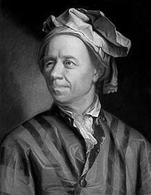
A protrait of Leonhard Euler by Emanuel Handmann, 1753.11.8
Euler's identity is one of the most famous and admired
equations in mathematics. It holds such an exalted status
because it uses the fundamental mathematical operations of addition,
multiplication, and exponentiation exactly once and it relates
several fundamental mathematical constants:
0, 1, ![]() , e, and i (the square root of minus one; the imaginary unit).
, e, and i (the square root of minus one; the imaginary unit).
Unfortunately, R does not appear to have such a high opinion of Euler's identity. In fact, R thinks that Euler is wrong!
> exp(pi*complex(im=1)) + 1 == 0 + 0i
[1] FALSE
What is going on? The problem is that it is not sensible to compare real values for equality. In this case, we are comparing complex values, but that boils down to comparing the real components and the real coefficients of the imaginary components. The problem is that the imaginary component of the left-hand side of the equation is very close to, but not quite exactly 0i.
> exp(pi*complex(im=1)) + 1
[1] 0+1.224606e-16i
This is an example where the all.equal() function can be used to compare real values and ignore tiny differences at the level of the precision of the computer.
> all.equal(exp(pi*complex(im=1)) + 1, 0 + 0i)
[1] TRUE
Hooray! Euler's identity is saved!
Paul Murrell

This document is licensed under a Creative Commons Attribution-Noncommercial-Share Alike 3.0 License.