![\begin{figure}% the gap below seems to be important!??
\par
\includegraphics[width=\textwidth]{script-worldpop}\end{figure}](img47.png) |
As early as the 1970s, Isaac Asimov was attempting to draw the eye of the general public to the looming problem of the overpopulation of Planet Earth. In several books and speeches11.1he dramatically pointed out that the world population at the time stood at around 4 billion, but with the increasing rate of growth, it would be around 7 billion by the turn of the millenium. Asimov also pointed out that, one way or another, the growth of the human population would slow, it was just a matter of how messy the deceleration was. Nature and the limits of natural resources would do the job if necessary, but the least messy solution, he suggested, was voluntary birth control.
Asimov did not live to see the turn of the millenium, but he may have been pleased to see that his prediction was slightly pessimistic, not because his calculations were wrong, but because population growth had begun to slow, and because it was slowing for non-messy reasons.
Overall estimates of the population of the world can be obtained from the U.S. Census Bureau.11.2Figure 11.1 shows estimates dating from 1900 and extending until 2050. This clearly shows the upward curve during the first three quarters of the 20th Century, but already a straightening and tailing off beginning as we pass the turn of the millenium.
|
This slowing in the growth of the world's population is mainly thanks to lower fertility rates (the non-messy solution), which is due to cultural changes such as people marrying later, and the greater availability and use of contraceptives. Even longer term projections by the United Nations suggest that, assuming trends in lower fertility continue, the world's population may actually stabilize at around 9 or 10 billion before 2500. Asimov, not to mention his descendants, should be thrilled.
Another population-related service offered by the U.S. Census Bureau is the World Population Clock (see Figure 11.2).
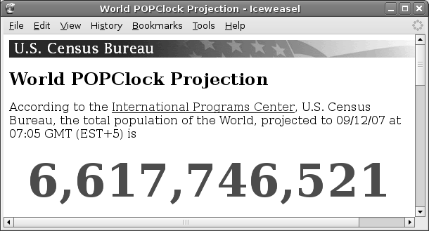 |
This web site provides an up-to-the-minute snapshot of the current estimate of the world's population, based on estimates by the U.S. Census Bureau. It is updated every few seconds.
What we are going to do in this section is to use this clock to generate a rough estimate of the current rate of growth of the world's population.
We will do this by looking at the steps involved, how we might perform this task “by hand”, and how we might use the computer to do the work instead. The steps involved are these:
What about getting the computer to do the work?
Navigating to a web page and downloading the information is not actually very difficult. The following code will do this data import task:
> clockHTML <-
    readLines("http://www.census.gov/ipc/www/popclockworld.html")
Getting the population estimate from the downloaded information is a bit more difficult, but not much. The first thing to realise is that we do not have a nice picture of the web page like we see in a browser. This is actually a good thing because it would be incredibly difficult for the computer to extract the information from a picture. What we have instead is the HTML code behind the web page (see Figure 11.3).
|
<!DOCTYPE html PUBLIC "-//W3C//DTD XHTML 1.0 Transitional//EN"
    "http://www.w3.org/TR/xhtml1/DTD/xhtml1-transitional.dtd">
<html xmlns="http://www.w3.org/1999/xhtml"
      xml:lang="en" lang="en">
<head>
    <title>World POPClock Projection</title>
    <link rel="stylesheet"
          href="popclockworld%20Files/style.css"
          type="text/css">
    <meta name="author" content="Population Division">
    <meta http-equiv="Content-Type"
          content="text/html; charset=iso-8859-1">
    <meta name="keywords" content="world, population">
    <meta name="description"
          content="current world population estimate">
    <style type="text/css">
        #worldnumber {
	    text-align: center;
	    font-weight: bold;
	    font-size: 400%;
	    color: #ff0000;
        }
    </style>
</head>
<body>
    <div id="cb_header">
    <a href="http://www.census.gov/">
    <img src="popclockworld%20Files/cb_head.gif"
         alt="U.S. Census Bureau"
         border="0" height="25" width="639">
    </a>
    </div>

    <h1>World POPClock Projection</h1>

    <p></p>
    According to the <a href="http://www.census.gov/ipc/www/">
    International Programs Center</a>, U.S. Census Bureau,
    the total population of the World, projected to 09/12/07
    at 07:05 GMT (EST+5) is<br><br>
    <div id="worldnumber">6,617,746,521</div>
    <p></p>
    <hr>
...
|
This is better than a picture because there is structure to this information and we can use that structure to get the computer to extract the information for us. The current population value is within an HTML div tag with an id attribute (line 41 in Figure 11.3). This makes it very easy to find the line that contains the population estimate; this is just a text search task. The following code is one way to peform this task:
> popLine <- grep('id="worldnumber"', clockHTML)
> popLine
[1] 41
It is also easy to extract the population estimate from the line by deleting all of the bits of the line that we do not want. This is a text search-and-replace task and can be performed using the following code:
> popString <- gsub('^.+id="worldnumber">', "",
                     gsub("</div>.*", "",
                          clockHTML[popLine]))
> popString
[1] "6,617,746,521"
Finally, we need to turn the text of the population estimate into a number so that we can later carry out mathematical operations. This is called data coercion and appropriate code is shown below (notice that we have to remove the commas that are so useful for human viewers, but a complete distraction for computers):
> pop <- as.numeric(gsub(",", "", popString))
> pop
[1] 6617746521
This example provides a classic demonstration of the difference between performing a task by hand and writing code to get a computer to do the work. The manual method is simple, requires no new skills, and takes very little time. The computer code approach requires learning new information (it will take substantial chunks of this chapter to explain just the code we have used so far), so it is slower and harder. However, the computer code approach will pay off, as we are about to see.
The following code will make the computer wait for 10 minutes:
> Sys.sleep(600)
> clockHTML2 <-
       readLines("http://www.census.gov/ipc/www/popclockworld.html")
> popLine2 <- grep('id="worldnumber"', clockHTML2)
> popString2 <- gsub('^.+id="worldnumber">', "",
                     gsub("</div>.+", "",
                          clockHTML2[popLine2]))
> pop2 <- as.numeric(gsub(",", "", popString2))
> rateEstimate <- (pop2 - pop)/10
[1] 146.6
As mentioned previously, computers are world champions when it comes to mindlessly repeating tasks, so the computer code approach will now pay off handsomely.
The computer code that will generate 10 population growth rate estimates is shown in Figure 11.4. As usual, the details of how this code works are not important at this stage. However, there are several important features that we should highlight.
|
checkTheClock <- function() {
    clockHTML <-
     readLines("http://www.census.gov/ipc/www/popclockworld.html")
    popLine <- grep('id="worldnumber"', clockHTML)
    popString <- gsub('^.+id="worldnumber">', "",
                       gsub("</div>.*", "",
                            clockHTML[popLine]))
    as.numeric(gsub(",", "", popString))
}

rateEstimates <- rep(0, 10)

for (i in 1:10) {
    pop1 <- checkTheClock()
    Sys.sleep(600) # Wait 10 minutes
    pop2 <- checkTheClock()
    rateEstimates[i] <- (pop2 - pop1) / 10
}

writeLines(as.character(rateEstimates),
           paste("popGrowthEstimates",
                 as.Date(Sys.time()), sep=""))
|
The core task in this example involves downloading the World Population Clock and processing the information to extract a time and a population estimate. For each estimate of the population growth rate, this core task must be performed twice. A naive approach would suggest writing out two copies of the code to perform the task. However, that would violate the DRY principle (see Section 2.11) because it would create two copies of an important piece of information; the information in this case being computer code to perform a certain task. As can be seen from Figure 11.4, the code can be written so that only one copy is required ( lines 2 to 8) and that single copy can be referred to from elsewhere in the code (lines 14 and 16).
At a slightly higher level, the task of calculating an estimate of the population growth is also repeated, in this case, 10 times. Again, rather than having 10 copies of the code to calculate an estimate, there is only one copy ( lines 14 to 17), with other code to express the fact that the this sub-task needs to be repeated 10 times (lines 13 and 18).
This chapter is concerned with writing code like this, using the R language, to perform general data handling tasks: importing and exporting data, manipulating the shape of the data, and processing data into new forms.
Paul Murrell

This document is licensed under a Creative Commons Attribution-Noncommercial-Share Alike 3.0 License.